A kept historical snapshot
The architecture, v1 (archived snapshot)
The frozen v1 architecture spec, superseded by the current spec at /architecture/. Kept as a historical snapshot so the page always shows the latest while nothing is lost: the depth-three apical-credit comprehension-and-abstraction core and the generation loop, before the two-engines reframe.
Architecture v1 (archived snapshot) - superseded by the current spec at /architecture/.
Architecture v1 · 2026-06-27 · the current canonical spec
This page is the architecture spec: the model the experiments have converged the code into, described in detail and explained. It is the counterpart to the lab notebook: the notebook is the running journal of every experiment; this page is the standing answer to "what is the kinogaki-cortex code, right now, and why is it shaped this way?" The architecture has two halves: a comprehension-and-abstraction core, which is locked and validated above the backprop ceiling, and a generation loop, just opened with its first positive. Experiments drive this page; when an experiment shifts the architecture, this spec is re-versioned and the change is logged at the bottom.
Overview
kinogaki-cortex is a brain-inspired model of text. It learns the way a person reads: online (every character teaches it, one pass, no retraining), gradient-free in regime (it learns on arrival without a global backward pass over the data), bounded-memory (it lives under a budget and must generalize to stay good), and guided by human cognition at every fork. Those are the four laws; they are not style, they are the constraints the whole program holds itself to.
The architecture is two halves, matching the two things a language user does: understand, and speak.
- The abstraction core, locked. A multi-level stack that reads a character context and predicts the next character, building an abstract, generalizing internal code as it climbs. The core is settled: it reaches a transfer abstraction score (CCGP) of 0.50 to 0.55, above the 0.484 backprop ceiling, stable and seed-robust. This half answers comprehension.
- The generation loop, opening. An internal self-feedback loop, the birdsong loop, that produces an utterance, re-comprehends its own output, and corrects toward what it intended, learning to speak with no listener. This half has its first positive (the internal half of generation); its external half, a referential game that fixes a shared convention, is the named next move.
The rest of this page walks the data path end to end: encoder, the abstraction core (level by level, with the apical credit wire and the stabilizers, and why each piece is there), the readout, and the generation loop, then states plainly what is deliberately not in the architecture.
The data path, at a glance
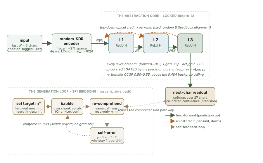
Two pathways, one set of counts read two ways: reading selects the next character for fidelity to the stream; speaking selects an utterance for what a re-hearing of it recovers. The forward (feed-forward) wires carry prediction up; the apical wires carry credit down; the same precision signal is read three ways: as attention/vote gain, as working-memory eligibility, and as the per-unit credit amplitude.
1 · Input: the random-SDR encoder
The model never sees raw characters. It sees a fixed-random sparse distributed code of the recent context.
The alphabet is 27 symbols: a to z are 0 to 25, space is 26. Each letter is assigned one fixed random sparse code (k active bits out of n, about 2% density) drawn once from a seed and never changed. There is no learning in the encoder; it is a frozen, deterministic dictionary (LetterSDR in lib/sdr_encoder.py).
The context window is the last W = 5 characters. To encode it, each of the five letters' codes is position-tagged (rolled by offset × stride bits, so the same letter in a different slot lands on a different bit set) and all five shifted codes are OR'd into one input SDR (ContextEncoder.encode). Position-tagging is what lets the layer above tell "the a two back" from "the a just now"; OR-ing keeps the input at a fixed size n no matter how wide the window, and makes similar contexts (sharing letters at the same offsets) share input bits, the overlap a pooler needs to map similar contexts to similar codes.
For the abstraction core the SDR is then taken dense and L2-normalized into one vector of dimension n_in = 1024 (featurize_dense in lib/mlx_learner.py). That normalized dense vector is the input to L1.
Why a fixed random code and not a learned embedding: a learned embedding would need a gradient, and the whole point of the core is to build abstraction without one. The random SDR is a high-dimensional, sparse, content-preserving substrate the stack can carve, exactly the role the brain's input projections play in the geometry the program is chasing (the PFC neural-geometry result grounds this: learning shapes the geometry from high-dimensional-random toward low-dimensional rule-selective).
2 · The abstraction core: the locked model
This is the heart of the architecture, and the part the experiments worked hardest to settle. In code it is StabilizedApicalStack (experiments/exp_dj_stability/arch.py), a thin, validated configuration over MLXApicalStack (experiments/lib/mlx_learner.py). The locked configuration is: depth-3, actnorm plus gate-clip, act_gain ≈ 0.2, the apical credit gated by precision. Every clause of that sentence was bought by an experiment. Here is the stack, piece by piece, with the reason each piece exists.
The shape: a depth-3 stack with a next-char readout
The forward shape is a straight climb. The input SDR (n_in = 1024) feeds L1 through W[0] (n_in × H); L1 feeds L2 through W[1] (H × H); L2 feeds L3 through W[2] (H × H); and L3 feeds the readout through Wo (H × n_out), a linear softmax over the next character (n_out = 27). That is the prediction path of the diagram above, traced level by level.
Three hidden ReLU levels (H units each, typically 768 to 1024), then a linear softmax readout over the 27 next-character classes. The forward pass is ordinary: each level is ReLU(input · W + b), the top level feeds the readout. What is not ordinary is how the weights learn: there is no backprop anywhere.
Why depth 3, and not more. Depth is what buys altitude: each level out-abstracts the one below, and abstraction (CCGP) climbs L1 → L2 → L3. But it climbs to three and then saturates: depth-4 adds dimensionality without adding abstraction, and the deep levels collapse. That ceiling was established by scaling the stack (three swings after the keystone) and confirmed when the capstone meant to push past it ran and failed (the architecture is locked). Three is the settled depth.
The apical credit wire: the abstraction itself
Between every adjacent pair of levels there is a second wire running the other way: a per-unit, top-down apical credit signal. This is the mechanism that makes the stack abstract, and it is the single most important idea in the core.
The readout's error is dz = p − onehot(target). That error is routed back into the hidden levels not through the transpose of the forward weights (that would be backprop, which needs weight transport, a neuron reading its own outgoing synapses, which biology cannot do), but through fixed random feedback matrices: B_top from the readout to the top hidden level, and an apical wire Bap[ℓ] (an H × H fixed random matrix) from each level to the one below it. This is feedback alignment: the credit each unit receives is per-unit and local, carried down a real top-down pathway, with no weight transport. The forward weight then takes a local delta step against that per-unit credit.
The credit flows level by level, top to bottom:
  dz   = p − onehot(target)
  Wo  -= fa_lr · outer(h_L, dz)              # readout: its own local delta
  d_L  = (B_top · dz) · [h_L > 0]            # top level: error → top hidden via fixed B_top
  W_L -= fa_lr · outer(h_{L-1}, d_L)         # train the top forward weight (ungated)
  for ℓ = L-1 … 1:                           # carry the credit DOWN, level by level (apical)
      d_ℓ  = (Bap[ℓ] · d_{ℓ+1}) · [h_ℓ > 0]  # per-unit credit from the level above
      d_ℓ  = normalize(d_ℓ)                  # RMS-normalize the credit (gate-clip)
      W_ℓ -= (ap_lr · g) · outer(in_ℓ, d_ℓ)  # GATED by the precision burst g
The same top-down wire that carries this credit is the wire that would prime the level below during a forward sweep: priming and credit are one mechanism. This is the architectural keystone, and the reason the core exists in this form.
Why per-unit, and why this pathway. The program walked the abstraction question all the way down. First it proved the missing ingredient was credit assignment, not wiring: holding one architecture fixed and swapping only the update rule, a gradient builds an abstract space while a no-gradient Hebbian rule compresses hard but loses abstraction (the abstraction wall was credit assignment). Then it sharpened "credit assignment" to per-unit credit: a broadcast neuromodulatory scalar fails (one number everywhere can only scale an unsupervised step), while a per-unit feedback-alignment signal clears the wall, lifting abstraction to ~0.41 and approaching the backprop oracle's ~0.49 (a local signal clears the wall). Then it answered on what pathway, how biologically: carry that per-unit credit down a real apical wire, and the result is the first stack whose abstraction climbs with depth (the apical fusion). The apical wire is not decoration; it is the abstraction.
The precision signal: the third factor that gates the credit
The credit does not flow at a constant rate. Its amplitude is gated by a precision/surprise burst, the third factor. On each step the model reads its own surprise on the true character, s = −log₂ p(target), tracks a running mean of it, and forms a bounded burst g = g_floor + clip(s − running_mean, 0, burst_max). The apical (below-top) updates are scaled by g; the top forward weight and the readout are left ungated, so the gate's effect is isolated to the apical wires.
This is the "one precision read three ways" principle: the same precision burst is (1) the attention/vote gain that sharpens confident columns, (2) the working-memory eligibility, and (3) the per-unit credit amplitude here. It says when to learn hard (on the surprising characters) while the per-unit feedback says how each unit should change.
Why gating is load-bearing, and why it had to be tamed. On a two-level stack, the gated apical fusion (transfer CCGP 0.501) decisively beat the ungated wire (0.355): without the precision "when," apical delivery actually underperformed plain single-layer feedback alignment. But at depth the gate flipped sign: it became the primary destabilizer, amplifying a runaway in the forward activations (three swings after the keystone). The fix was not to drop it but to bound its range (gate-clip; see below). Precision-gating stays in the locked stack, range-limited.
The stabilizers: actnorm and gate-clip, what stops divergence
Feedback alignment, stacked with a precision gate, diverges at depth without help: the forward activations grow unbounded (one level's RMS runs away from ~0.02 to tens), the credit is an outer product of those activations so it blows up too, and the surprise gate amplifies the runaway. Stability, not depth, not data, was the wall. Two pieces, applied to every level, solve it.
- actnorm, forward-RMS normalization. After each level's ReLU, the hidden vector is rescaled to a fixed target RMS,
act_gain(hidden_levels_mxinarch.py). This is homeostatic gain control: the forward can no longer blow up, so the credit stays bounded too. The target RMS is set to the healthy early-training scale (about 0.1, not unit-RMS; unit-RMS would itself inflate the forward and destabilize). actnorm is necessary and sufficient for stability: it holds the stack stable at every depth, rate, and data size where the baseline, a gate-clip alone, and a dream-replay cycle alone all diverge into the teens of bits-per-char (the architecture is locked). - gate-clip, bounded precision burst plus RMS-normalized credit. Stability is not abstraction: plain actnorm stays stable but collapses the deep code to one dimension (its high score is a degenerate-code artifact). Gate-clip keeps the code healthy: it tightens the gate's ceiling (a smaller
burst_max) and RMS-normalizes the apical creditdto a fixed scale before the gated step, so no single level's update can blow up regardless of the gain (_gateclip_stepinarch.py). With both pieces, the depth-3 stack reaches transfer CCGP 0.508 to 0.549, above the 0.484 ceiling, with healthy dimensionality, on both seeds.
Both are required: actnorm for stability, gate-clip for an abstraction that is real rather than collapsed.
act_gain ≈ 0.2: the sharp peak
act_gain (the actnorm target RMS, which doubles as the precision-gain dial) is a unimodal, sharply-peaked knob. A gain of 0.1 lands just under the ceiling (~0.449); a gain of 0.2 hits the peak, about 0.50 to 0.55, above the ceiling, seed-robust; a gain of 0.3 or more over-drives the stack and the deep code dies (collapses to one dimension). The locked configuration sits on that peak.
The headline result
Put together (depth-3, per-unit precision-gated apical credit, actnorm plus gate-clip, act_gain ≈ 0.2) the core produces what every prior gradient-free stack in the program failed to produce: rising-altitude abstraction. CCGP climbs L1 → L2 → L3, the transfer score reaches 0.50 to 0.55, above the 0.484 single-layer backprop ceiling, and it is stable and seed-robust. This is a biologically-shaped, online, local, bounded learner that builds an abstract code without a gradient, the named prize of the abstraction line, in hand.
3 · Readout: comprehension and calibrated confidence
The top hidden level feeds a linear softmax over the 27 characters: that is the next-character prediction, the comprehension output. The readout learns by its own local delta against dz (no transport).
Alongside the prediction the model exposes a calibrated confidence, the precision read. A count split into hits and misses gives a NARS truth value (f, c) whose product f·c is calibrated essentially for free (how sure is a count?), and this is the same precision/surprise signal that gates the apical credit. So the readout emits two things: what comes next, and how sure the model is, and that confidence is not a separate module, it is the third factor read off the prediction itself.
4 · The generation loop: SF1, the internal half (nascent)
With the core locked, the program's open value moved to generation: producing text, not just modelling it. Generation has two halves; the internal half just landed its first positive in experiments/exp_sf1_selffeedback/run.py, the birdsong loop. A songbird learns its song from self-hearing alone, with no tutor present: it babbles, hears itself, and corrects toward the song it means to sing. SF1 builds that loop for text. It is online, gradient-free, bounded, and needs no environment.
One iteration of the loop:
- Set the target. An intended meaning
m*(a real held-out word the comprehension pathway already represents) is fixed, and is set independently of the producer (the anti-trivial-fixed-point guard). The meaning is stored as a salience-weighted "heard fingerprint," not a raw string, so the producer cannot cheat by string-matching; it must produce something that sounds like the meaning to comprehension. - Babble. The producer samples candidate utterances over the AU committed-chunk emission vocabulary (
ChunkLexicon), whole committed units, not characters, biased by its learned per-meaning chunk counts plus an explore term that anneals down as competence rises (subsong → song). - Re-comprehend. The same comprehension pathway reads each candidate utterance and recovers a posterior
m̂over meanings, the forward model pointed inward. This pass is read-only: it never writes the comprehension counts (attenuation). - Self-error.
e = 1 − m̂[m*], one minus the mass the re-comprehension puts on the intended meaning. The NARSf·cconfidence on the utterance is logged as a cheap second view (the self-monitor). - Correct, win-stay / lose-shift. A small error reinforces the chunks that were used (win-stay); a large error weakens them (lose-shift). The self-error is consumed as a scalar reward by count reinforcement: no gradient is routed back through the comprehension decoder.
So the agent produces, re-comprehends, scores itself against the target, and revises, all inside one cortex, the only learning being count reinforcement on a self-generated error.
The result. Against a chance of 0.042 (one of 24 meanings), the full loop recovers an intended meaning 0.271 of the time: about 6.5× chance and 8× its own open-loop and deafened ablations (which sit at chance with zero coverage). All three guards fire: scramble the target and it collapses to exactly chance; let the self-output contaminate comprehension and an independent frozen judge catches the private-code drift (it fools its own ear, buys no real production). So internal self-feedback teaches production with no listener: self-practice teaches fluency and form (the generation frontier, opened).
The honest scope. Absolute recovery (~0.27 on 24 meanings) is modest, a first cut on a coarse meaning code and a simple count re-hearer. And by design the loop only ever agrees with itself: it supplies fluency, not a shared convention. Convention needs the external half: a referential game (the planned audience-model / listener-table work) scored on whether a real listener recovers the referent, the anchor against private-code drift. The internal half is in the black; the external half is the falsifiable next move. The loop is the architecture's nascent speaking organ; the core is its settled understanding organ.
5 · Attention and working memory: a validated subsystem
A second altitude rides on top of the prediction columns: a learned attention system that decides where each column looks and what the level above holds while it reads. The whole stack is online, gradient-free, and bounded, and at the payoff scale it beats hand-set fixed views. It came together over three experiments, each adding the one piece the last one named, and it now stands as a validated subsystem.
The encoder above reads a fixed window a fixed distance back. The attention subsystem makes that distance a choice. Each column reads a view, a window a chosen distance back over a fixed span, and the attention is the policy that picks the distance.
- Each column learns where to look. The look-back offset is an action, chosen fresh every step and rewarded by how well the column then predicts, the program's "motor is moving through text" made concrete. A count-based, gradient-free bandit over a menu of offsets learns the choice, the menu holding one content-relative word-jump (look back to the previous word boundary). The wire that makes it work is lateral inhibition on the action space: a column is docked for predicting well where the other columns already look, the same diversity pressure that clears the representational collapse, carried from the code to the scan. Without it every column collapses onto the single most recent character and prediction explodes; with it the columns spread across complementary offsets (learning where to look).
- A higher level guides the scan by context. Context-free, the learned scan only ties the hand-set spread, because with no context to condition on a fixed spread is already good and free. So a working memory one level up steers it. The working memory is a leaky char-distribution over the region recently read plus the live word-phase, the running theme and the sentence-start held while the lower level reads the end. Each column's offset bandit is keyed on it, one value vector per context bucket, so the column learns in context X, look at offset Y. At the right granularity this beats the hand-set baseline on prediction, and it lifts the abstraction score (transfer CCGP) at every granularity, where the context-free round left abstraction flat. The scan is genuinely context-dependent, looking in different places in different contexts (where you look depends on what you understand).
- A gate decides when to update the held theme. The working memory began as a fixed leak, taking in a little of every character with no say over when. A basal-ganglia-style Go/NoGo gate replaces the leak. It fires on a model-update signal, how far the column pool's own next-character prediction moved from one step to the next (the total-variation distance between consecutive pooled distributions), not raw surprise: the shift in the prediction carves events where raw surprise carves words. An adaptive tail threshold fires Go when the signal is in its high tail, self-calibrating, learned online and gradient-free with no reward. On Go the theme admits the current character; on NoGo it is held. At the payoff scale the gate beats the fixed leak (3.069 bits per char against 3.083) and the hand-set baseline (3.101), and it beats both degenerate bounds, always-update and never-update, so the win is the timing of the update and not the amount of theme motion. It fires about a fifth of the time, holds the theme roughly eight characters at a stretch, and fires at or next to a word boundary three times in four (a gate for working memory).
Put together, the full stack, columns learning where to look, guided by context from a higher level, holding the theme behind a learned gate, beats hand-set fixed diverse views, online and gradient-free, at the two-hundred-thousand-character scale.
The honest scope. This subsystem runs on the diverse-views count columns, a distinct substrate from the locked abstraction stack of section 2. The abstraction core is the single-column apical stack, settled above the backprop ceiling; the attention subsystem is the multi-column count bank, where diverse views are the prediction organ. They are separate organs, and the attention result is validated on its own substrate and scale, not yet fused into the locked core. The open items are recorded as the next round: a gate that targets a fire-rate directly (a fixed threshold under-fires as the data grows), and a deeper hierarchy of held states above the one theme (the L3 and L4 altitudes), the path to holding context across a long span. The numbers are the direction at this scale, three seeds, one count substrate, not a scaled benchmark.
6 · What is deliberately not in the architecture
The core is a single column. Several validated mechanisms are deliberately kept out of it, because the experiments factored the architecture cleanly and each of these belongs to a different job. Stating this plainly is part of the spec: the honesty bar is as load-bearing as the wins.
- Multi-attention / breadth is out of the abstraction core. Different attended views per column, pooled and precision-weighted, decisively help prediction (different views beat same views at every scale; same-view voting is worse than a single column) and keep the code high-dimensional. But they leave abstraction flat: breadth raises dimensionality without raising CCGP. So prediction and abstraction factor: prediction from diverse precision-weighted views, abstraction from per-unit apical credit (three swings after the keystone). The multi-column machinery exists in code (
MLXMultiColumnApicalStack) as the prediction organ, but the locked abstraction core is the single-column stack. - The breadth × stability combine ran and failed; the levers are not additive. It was natural to expect breadth (which keeps dimensionality high across columns) to rescue actnorm's deep collapse (which kills dimensionality across stimuli within a column). The "A1" capstone tested exactly that and the prediction was false: the combine stays stable but collapses to dimensionality 1.17, because the two levers act on different axes of variance and concatenation cannot undo a per-lane cross-stimulus collapse (the architecture is locked). The architecture is therefore locked at the depth-3 single-column winner, not at a combined stack.
- Deeper than 3 saturates. Depth-4 adds no abstraction (the stack is already at the ceiling at depth-3) and the deep levels collapse even when stable. Pushing past three needs a genuine design change (a soft forward bound that prevents divergence without pinning the activation magnitude, top-level-only normalization, or an ungated dimensionality-preserving regime) of uncertain payoff, since we are already at the ceiling. It is an open residual, not a closed door, and it is recorded as such.
- The drift on a long fresh stream is mitigated, not solved, so the mitigation stays out of the locked core. The locked config holds above the ceiling on a bounded corpus, but on a long fresh non-stationary stream it drifts: held-out bits-per-char rises and the deep code collapses toward rank one. Two mechanisms push that back, lateral divisive inhibition between same-level columns and K-line replay reinstated at an interior altitude, and they compose: at three million characters, with both on, the deep code stays high-dimensional, above the 0.484 ceiling at every checkpoint, and stable, where the bare config and each mechanism alone collapse on a different axis. The ten-million confirmation qualifies it. The mitigation is real (the bare config collapses to rank one with bits-per-char 4.120 and abstraction 0.317 by seven million; with both wires on the deep code survives, dimensionality 1.83 alive, bits-per-char 3.694, abstraction 0.429, stable), but partial and degrading at scale: the deep code stays alive, yet abstraction slips below the backprop ceiling (0.429 against the three-million run's ~0.56 above it) and the deep dimensionality is marginal. So the drift is mitigated, not cured, and the two wires are kept out of the locked core until a tuned, multi-seed run holds the protection above the ceiling at scale. It is an open continual-learning residual, recorded as such.
- A label-attractor shortcut to abstraction was ruled out. A self-supervised label-anchored prototype pull compresses dimensionality harder than anything in the line (PR 5.8) but scores below the raw baseline on transfer: compression is not abstraction. The gradient-free route to abstraction is per-unit credit, not a label attractor (three swings after the keystone).
Version history / Changelog
The architecture's evolution, newest first. Each entry is a published version; prior full versions are kept as snapshots (/architecture-v<N>/) so this page always shows the latest while nothing is lost. When an experiment shifts the architecture, this spec is re-versioned: the current full spec is copied to a /architecture-v<N>/ snapshot, this page is rewritten as the new full version, and an entry is appended here noting what changed and which experiment drove it.
- v1 · 2026-06-27 · initial architecture spec. The first canonical spec, written after the abstraction core was locked above the backprop ceiling (experiments DC → DE → DH → DI/DJ/DK/A1) and the generation loop opened with its first positive (SF1). Covers the random-SDR encoder, the depth-3 per-unit precision-gated apical-credit core with actnorm plus gate-clip at act_gain ≈ 0.2, the calibrated readout, and the internal self-feedback generation loop, and states what is deliberately kept out of the single-column core (multi-attention/breadth as a prediction organ, the non-additive breadth × stability combine, depth past 3, the label-attractor shortcut). No prior snapshot exists yet; this section is seeded with v1.
- note · 2026-06-28 · no version bump. The ten-million confirmation of the drift-mitigation compose (experiment SYNTH, the lateral-inhibition plus interior-replay pair) came back partial: it keeps the deep code alive on a long fresh stream where the bare config collapses, but abstraction slips below the backprop ceiling by seven million, so the drift is mitigated, not cured. The two wires stay out of the locked core; the "what is deliberately not in the architecture" section records the residual. No spec change, hence no version bump.
- note · 2026-06-28 · attention and working memory added as a validated subsystem (experiments AT1 → AT2 → AT3). The attention track closed its arc: columns learn where to look with lateral inhibition on the action space (AT1), a higher level guides the scan by context (AT2), and a basal-ganglia-style gated working memory holds the theme and updates it at boundaries (AT3), the full stack beating hand-set fixed views online and gradient-free at the two-hundred-thousand-character scale. Section 5 now describes it, with its honest scope: it rides the diverse-views count substrate, distinct from the locked single-column abstraction stack, and the open items are a fire-rate-target gate and a deeper hierarchy of held states. The new section sits alongside the existing spec rather than rewriting it, so no snapshot or version bump yet; the subsystem is a candidate for a v2 bump on review, once it is fused with or measured against the locked core.